I started off 2015 with an analysis of effective time in the J-League and which teams appeared to have a strong influence on it.  To start off 2016 I do the same type of analysis but from a Bayesian perspective.  My objective for 2016 is to take my analytics into more of a Bayesian direction — present not only point estimates but also uncertainties and probabilities in a more systematic way.

These data are collected as part of an initiative by the J-League called Plus Quality, which attempts to assess and improve the quality of their on-field product, from increasing playing time to decreasing time lost due to negative events.  Plus Quality started in 2013 and involves all league matches in the J-League’s three divisions, plus the League Cup matches.

Here’s some summary data on effective playing time in the 2015 season:

• The mean effective playing time in J1 matches was 3270 seconds, or 54 minutes 30 seconds.  This represents a 109 second decrease over last year’s competition.
• Standard deviation in J1 matches was 330.2 seconds, or 5 minutes 30.2 seconds, which is a 50 second increase over J1 matches in 2014.
• Match with most effective playing time: Kawasaki Frontale vs Sanfrecce Hiroshima (69 minutes 33 seconds, round 10 of 1st stage)
• Match with least effective playing time: FC Tokyo vs Matsumoto Yamaga FC (40 minutes 36 seconds, round 12 of 2nd stage)

The goal of this and previous analyses has been to identify the impact of clubs on the effective playing time relative to an average match.  The idea is that some teams are associated with playing styles and behaviors that either increase or reduce the amount of time that the ball is in play.  It’s a crude model to be sure, but one that describes the differences between certain teams.

Below is a plot of the club impacts on effective playing time.  The dot in the middle of the bar represents the median value of the club impact, and the lines extending from it represent the interval where we are 95% certain that the true club impact value lies (95% credible interval).  As was the case in the 2014 season, the presence of Sanfrecce Hiroshima in a J1 match adds between four and seven minutes to the effective playing time, while the presence of promoted side Montedio Yamagata subtracted between 2.5 and 5.5 minutes from the effective playing time.  Compared to last season, there doesn’t seem to be much turnover among teams in either half of the club impact chart, with the exception of Urawa Reds and Yokohama F-Marinos.

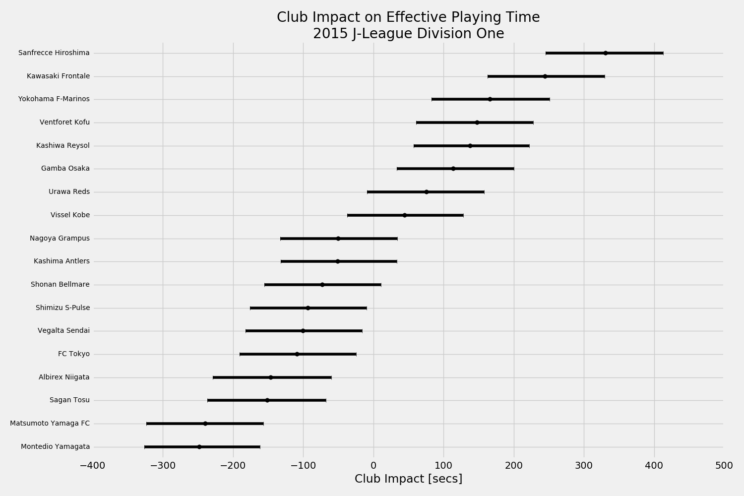
Club influence on effective playing time in 2015 J-League Division 1 matches.

I’ve added the J-League effective playing time data to the ProjectData repository on GitHub, and I’ve also included an iPython notebook of the Bayesian analysis so that you can check my work and perhaps extend it.

Appendix: Describing the Bayesian regression model

Here’s where I define the Bayesian regression model.  There’s math involved, so if you don’t want to see it, feel free to move along.

The Bayesian regression model is similar to the classic (frequentist) model in that you have an equation like this:

\[
y = \beta X + \epsilon
\]

Here, \(\beta\) represent the parameters, \(X\) the predictors, and \(\epsilon\) the unmodeled error.  The difference is that the data \(y\) is assumed to be drawn from a normal process and the parameters have prior probability distributions associated with them:

\begin{eqnarray}
y & \in & N\left(\beta X, \epsilon\right) \\
\beta & \in & N\left(\mu, \tau\right) \\
\epsilon & \in & N\left(0, \tau_e\right)
\end{eqnarray}

The priors of the parameters are updated with data \(y\) to yield posterior distributions, from which we can take samples and estimate the likely values of the parameters given our data.

In the case of effective playing time, the regression model is:

\[
T_{ij} = \beta_0 + \beta_i x_i + \beta_j x_j + \epsilon
\]

where the indices \(i\) and \(j\) represent home and away team indices, respectively, \(\beta_0\) the nominal match time, \(\beta_i\) and \(\beta_j\) the team impacts on effective playing time, and \(T_{ij}\) the effective playing time of the match involving teams \(x_i\) and \(x_j\).

The priors of the parameters are defined:

\begin{eqnarray}
\beta_0 & \in & N\left(\bar{T}_{ij}, 0.0001\right) \\
\beta_i & \in & N\left(0, 0.0001\right) \\
\epsilon & \in & N\left(0, 0.0001\right)
\end{eqnarray}

where \(\bar{T}_{ij}\) is the average effective match time over all league matches.