At this time last year I was reviewing a paper by Tim Swartz and his students on MLS draft pick valuation models.  Much has happened since then, such a couple of presentations in Vancouver and Atlanta on my own research on draft valuations.  With the MLS SuperDraft quickly approaching I’d like to summarize my work and its applications.

What’s a draft pick worth?

A draft pick is an asset that can be exercised, sold, traded, or allowed to expire unused.  With that in mind, it’s of interest to know what a draft pick is worth.  You could respond that the draft pick, like an illiquid or intangible asset, is worth what a willing buyer and seller agree upon, and that’s true.  A draft pick’s value can also be defined from the value of transactions involving a draft pick, or from the value (however we define it) of previously selected players at similar times of the draft, or any other method. We’d expect the top overall selection to be the most valuable because it provides a chance to select from the entire draft pool, and selections in an early round have more value than selections in later rounds.

What can we do with draft pick value?

Let’s say we agree upon a valuation of every slot in the draft.  There are a few things we can do with that information.  We can create a chart of the relative value of all draft picks to inform transactions involving a draft selection (which the Dallas Cowboys made famous).  We can combine the absolute value of these picks with projected values of candidate players to determine the best players available at a certain draft position.  If we go further and create values for every slot in previous drafts, we can go back and understand which draft selections in hindsight were clever or foolish, and which organizations were historically brilliant or suspect in their draft performance.

A valuation represents one perspective for defining value.  We could define draft pick value from career performances of past players or from what is offered in exchange for players, money, or other picks, which we could use to determine if one party is over- or under-estimating draft values, in our opinion.

Prior Art

Other analysts have considered the draft valuation problem and made their own contributions to it.  Tim Swartz and his team in the aforementioned paper created valuation curves by making lowess (local regression) fits of peak salary levels and minutes played as a function of draft position over a 12-year period.  Ford Bohrmann also used a lowess fit of career minutes played by drafted players to create his valuation model.  A contributor to the Sounder At Heart website charted a moving average of minutes played by draftees in four consecutive SuperDrafts in order to identify over- and under-performing draft selections and organizations.  There are others who have attempted to identify draft performance through descriptive statistics or their own scoring systems.

Contributions

There are some things about this analysis that make it stand out against the prior art:

• It covers almost the entire history of the MLS College and Super drafts, from the 1997 College Draft to the present day. (Supplemental Drafts are not considered but dealt with separately.)
• Every player selected by the MLS draft is incorporated in this analysis — over 1,700 players.
• Draft pick valuation models are created that are valid only for a specific MLS season (except the first one), and incorporate player data from the previous four seasons only.
• As an alternative to local regression, a Bayesian regression is applied to the data in order to determine credible bounds of expected draft values.
• Create two types of valuation models that communicate the following: the ability of clubs to identify talent able to thrive in the league, and the ability of clubs to find talent that benefits them.

Valuation Models

There are a couple of things that we have to define before we formulate valuation models.  Here they are below.

Normalized draft position

The number of slots in MLS’ drafts has changed significantly over the years, from 160 picks over 16 rounds in the 1996 Inaugural Draft to 88 over four rounds this year.  We transform the draft position \(i \in [1, N]\) so that it lies on a \(\alpha \in [0, 1]\) interval — draft position 0 is the first pick, and draft position 1 is the final pick.

\[
\alpha  = \frac{i – 1}{N – 1}
\]

Player value formulation

This will be controversial, and I recognize that it’s imperfect, but I chose to create a simple measure of career value using summary statistics that are accessible in every MLS season:

\[
V = \sqrt{\left(\frac{M}{M_{max}}\right)^2 + \left(\frac{G}{G_{max}}\right)^2 + \left(\frac{A}{A_{max}} \right)^2}, \, \mbox{field players}
\]

\[
V = \sqrt{\left(\frac{M}{M_{max}}\right)^2 + \left(1 – \frac{G_A}{G_{A, max}}\right)^2 + \left(\frac{S}{S_{max}} \right)^2}, \, \mbox{goalkeepers}
\]

The basic idea is that I wanted to capture player participation (minutes played) and player performance (goals scored and assists made for field players, goals allowed and clean sheets for goalkeepers).  All of the metrics are scaled by the league leaders in respective categories.  Goals allowed is a “negative” metric, so a low number relative to the league maximum is seen in the same way as being among the league leaders in goals or assists.

A more robust metric such as adjusted plus-minus or points above replacement can be dropped in place of the above metrics, but this simple value allows us to compare drafts across the entire history of MLS.

Draft performance rating

As I wrote before, one of the applications of a draft valuation model is to evaluate past draft selections.  To this end I’ve created an expression that scales the difference between and expected and actual career value by the normalized draft position.  The idea is that late selections that go on to make significant contributions should be strongly weighted positively, and early selections that turn out to be duds should be strongly weighted negatively.

\[
R = \Delta e^\alpha,\, \Delta > 0
\]

\[
R = \Delta e^{1-\alpha},\, \Delta < 0
\]

Valuation algorithms

Essentially the valuation model is a function that relates the draft position to its expected career value:

\[
V = f(\alpha)
\]

Our goal is to determine \(f(\alpha)\), and from there, estimate the career value associated with a draft pick.

One method to determine \(f(\alpha)\) is a lowess regression, which is a locally-weighted and smoothed linear regression.  This is what Swartz et al. and Bohrmann used to estimate their valuation curves.  It’s non-parametric, so the resulting curve can’t be described easily by an equation.

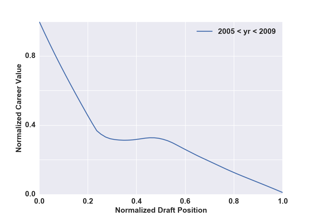
Normalized draft value curve valid for 2009 MLS SuperDraft, using data from players drafted 2005-2008.

The other method is a Gaussian process model, which is a non-parametric Bayesian regression model.  We assume that the points that make up the curve are drawn from a multivariate Gaussian distribution with zero mean and variance defined by a covariance matrix.  It’s this covariance matrix that defines the amount of continuity and smoothing in the resulting curve.  A fuller description of the model is in my Atlanta presentation slides, but the main idea is that we can produce uncertainty regions around the expected draft value curve.

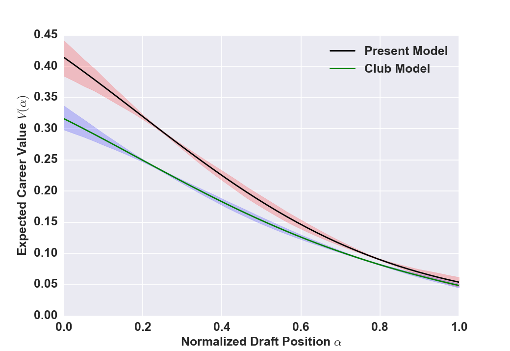
Draft value models effective for 2009 MLS SuperDraft using a Bayesian approach. Solid lines are median values, shaded areas are 95% credible regions.

Types of valuation models

The valuation models are trained with the career values calculated for all players drafted in the College Draft or SuperDraft.  The scope of the training data determines the model’s type.  I’ve defined two models — a “Present Model” and a “Club Model.”

The Present Model is trained with cumulative player value data of draftees the four years before the year of interest — a 2009 model is built with data from players drafted between 2005-2008.  Even if a player goes on to have a longer career, we only consider his performance in those four years.  The reason is that in 2009, we’re not aware which drafted players will go on to long career in MLS, so we can only work with the knowledge available at that time.  It’s “living in the present”, which inspired the name of this model.

The Club Model is similar to the Present Model, except that the cumulative player value data is calculated only for the period where the draftee is playing for the club that drafted him.  The thinking is that clubs are more interested in drafting players who will best benefit them than players who are likely to have long and productive professional careers.

There is a significant difference between the valuation curves associated with both models.  It’s especially pronounced in early draft picks and in previous MLS seasons before 2011.

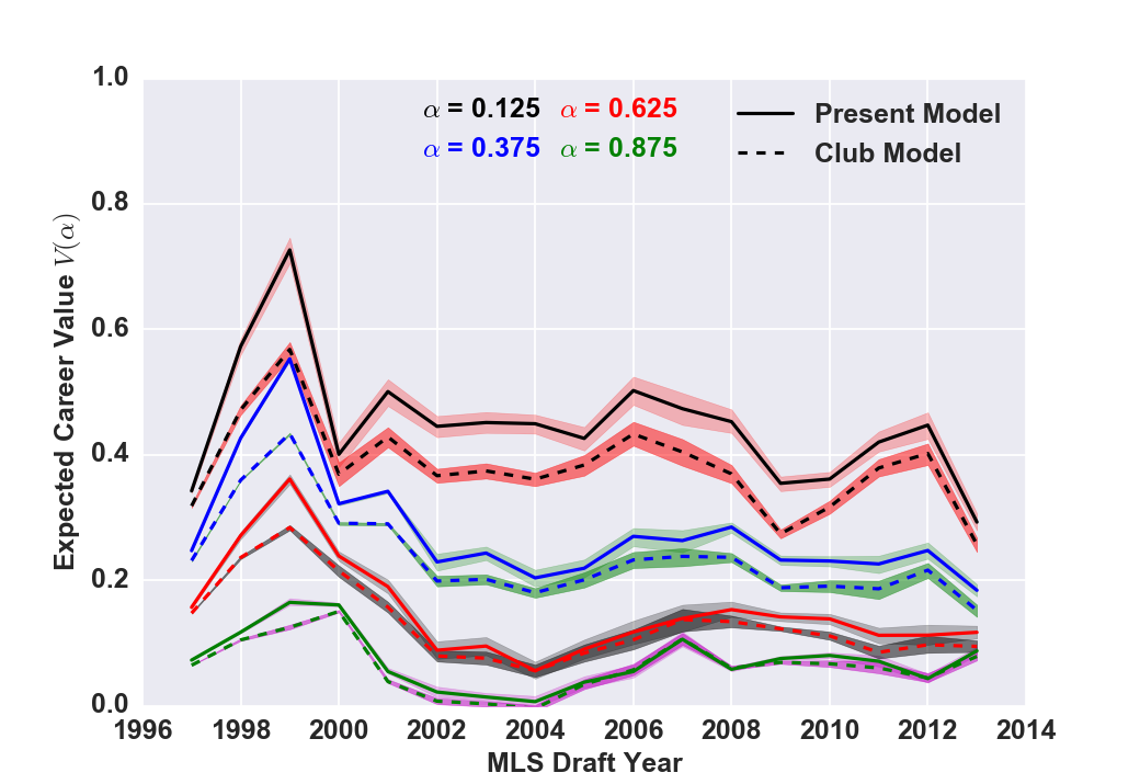
Comparison of expected career value of draftees from Present and Club draft valuation models, valid for MLS College/SuperDrafts between 1997 and 2003.

So why apply a four-year window?  From my survival analysis of MLS draft classes, the median lifetime of a draft class is four seasons, so that seemed like a reasonable cutoff.

To be continued

This post is getting way too long and I want to publish part of it now, so I’ll stop here and create Part 2 later.