Adjusted Plus/Minus in football – why it’s hard, and why it’s probably useless
Categories: Player Performance
It’s been several years since I’ve last written about the adjusted plus/minus problem in soccer — almost four years ago in fact. I had given a link to early work done by the late Climbing The Ladder blog and referenced a couple of presentations by researchers at conferences (Joe Sill and Wayne Winston), but said that I would present my own thoughts on the subject and never did. It’s time to revisit the topic.
Why Adjusted Plus/Minus?
Plus/minus rating is a simple concept — identify a player’s implied effect on his team’s goal difference while he is on the field of play. Adjusted plus/minus attempts to establish this contribution while accounting for the player’s teammates and the team’s opponents on the field.
A player’s effect on his team’s goal differential will change as the makeup of teammates and opponents changes during the game, but if you look at a large number of scenarios it should be possible to come up with a measure of how each player contributes to the game. It follows that if you know what each player contributes to the game’s outcome, it should be possible to look at the 22 players on the field and predict the expected margin of victory. So the adjusted plus/minus should serve as not only a descriptive model, but a predictive one as well. Such as it is, I’m very skeptical about the latter and I’ll explain why later.
What makes the adjusted plus/minus so attractive is that the data required to compute it are already available. One needs only the player lineups, substitutions and expulsion records with the times at which they occurred, and goals scored and their times. This metric should provide the opportunity to calculate ratings for any league with match details, therefore providing a chance to evaluate previous years and even decades.
Prior Art in Soccer Plus/Minus
I’ve already mentioned the plus/minus work by the Climbing the Ladder blog, and since 2010 I could only find a couple of posts on plus/minus in football.
There is this post by Omar Chaudhuri of 5 Added Minutes (now at Prozone Sports) who criticizes Opta’s use of what I’d call “naive” plus-minus that is uncontrolled for teammates and opposing players.
There is also a post by Ford Bohrmann which attempted to implement a simple adjusted plus/minus on 2010-11 English Premier League data. The resulting coefficients of the players were statistically insignificant from zero, which isn’t very interesting. Ford didn’t say if he had split the dataset into randomized training, validation, and testing groups. If he had, I am very confident that his results would have changed with each run, which would imply that the results are insignificant and unstable.
A third site called GoalImpact calculates the implied influence of a player on the goal difference of his team while he is on the pitch. The algorithm is described in such a way that it has to be something similar to an adjusted plus/minus formula.
The Adjusted Plus/Minus Model
I stated earlier that adjusted plus/minus is the goal difference associated with a player while controlling for the presence of the player’s teammates and opponents. I control for teammates and opponents using a linear regression model, which is described below:
\[
90\frac{\Delta G}{M_j} = \alpha_0 + \alpha_1 x_1 + \alpha_2 x_2 + \ldots + \alpha_i x_i + \ldots + \alpha_N x_n + e
\]
with the following terms:
- \(\Delta G\): Goal margin, \(G_{home} – G_{away}\)
- \(M_j\): Length of time segment, the interval in which no substitutions or expulsions occurred, for \(j = 1, \ldots, R\) segments [in minutes]
- \(\alpha_0\): Average home advantage over all teams in competition
- \(\alpha_i\): Influence of player \(i\) on goal differential, for \(i = 1, \ldots, N\) players in competition
- \(x_i\): Player appearance index:
- +1: Player \(i\) is playing at home
- 0: Player \(i\) is not playing
- -1: Player \(i\) is playing away
For the moment, players sent off are assigned an appearance index of zero for the remainder of the game, but one criticism of this approach is that it fails to assign some sort of penalty for placing his team at a numerical disadvantage. This type of accounting is challenging to implement, and I haven’t come up with a solid implementation scheme until very recently, so I’ll leave it alone for now and return to it in a future post.
So Why Is Adjusted Plus/Minus Hard?
Like a lot of problems in advanced soccer analytics, adjusted plus/minus is hard because of two nontrivial issues: data manipulation and algorithm development.
It’s true that all the data needed to create an adjusted plus/minus model are publicly available, but those data must be used to split each match into segments in which all of the players on the pitch are unchanged. One must repeat this process for every match in the competition. The least painful way to create these segments is by querying a database. (Incidentally, this functionality is now part of the Soccermetrics API.)
Algorithm development is the next nontrivial issue. The typical procedure for a regression model is to solve it using an ordinary least squares algorithm. The objective is to minimize the error between the observed value (our vector \(y\)) and the estimated value (our system matrix \(A\) multiplied by the estimated parameters). In other words:
\begin{eqnarray}
\min_x || \mathbf{A}x – y ||^2_2 \\
x^* = \left(\mathbf{A}^T\mathbf{A}\right)^{-1} \mathbf{A}^T y
\end{eqnarray}
Adjusted plus/minus belongs to the class of math problems called inverse problems which are characterized by ill-defined system matrices. The result is that the parameters that one wants to estimate have a lot of numerical noise, so they either have huge standard errors that renders them insignificant from zero or they just can’t be calculated because of a singular matrix.
There is a large class of methods that regularize, or stabilize, the system matrix, of which Tikhonov regularization (aka ridge regression) is most popular. Tikhonov regularization makes a trade-off between minimizing the estimation error (suppressing noise) and minimizing the magnitude of the estimate (risking loss of information):
\begin{eqnarray}
\min_x || \mathbf{A}x – y ||^2_2 + || \lambda x ||^2_2 \\
x^* = \left(\mathbf{A}^T\mathbf{A} + \lambda^2 \mathbf{I}\right)^{-1} \mathbf{A}^T y
\end{eqnarray}
The tradeoff between signal and noise is expressed in the Tikhonov parameter \(\lambda\). Nowadays with software packages such as R and scikit-learn one can automate much of the model fitting and testing, but inverse problems do require considerable amounts of careful treatment.
Modeling Procedures
It’s time to test this model on real data, and for my demonstration case I used the 2011-12 English Premier League match data that is contained in the public beta of the Soccermetrics API. I used the players and match segment resources of the API to build the matrices that form the plus/minus model and then split the matrices into two sections. One section (30 matchdays, or 300 matches) would be used to train and validate the model; the other section (8 matchdays, or 80 matches) is reserved solely to evaluate the selected model parameters. Over the two sections, there are 2144 segments involving 539 players in the 2011-12 Premier League.
To estimate the parameters in the adjusted plus/minus model, I use a technique called k-fold cross-validation (CV). K-fold cross-validation splits the dataset into groups, or folds, and combines all of the folds except one which is reserved for validation. This is repeated k times and the estimation results from each run are averaged. For this modeling I use 8 folds and two different regression algorithms: the ordinary least squares technique, and a ridge regression using a \(\lambda\) which minimizes the RMSE on the test data set.
Adjusted Plus/Minus Results
Ordinary least squares
Let’s start with adjusted plus/minus results using ordinary least squares. Here are the top twenty players in terms of adjusted plus/minus:
| Player | APM | Std Error |
| Leighton Baines | 2275017294229.67 | 11366509484918.9 |
| Brad Friedel | 1429320370141.13 | 9414634111710.74 |
| Joe Hart | 1400909544367.58 | 8336064683520.71 |
| Micah Richards | 1350995176838.36 | 8513987423148.42 |
| Kolo Touré | 1273699247132.48 | 6188264761376.42 |
| Nick Blackman | 1111264954722.86 | 5341199873841.63 |
| Luka Modrić | 1101085433727.49 | 7730040116309.95 |
| Piscu | 1029247309242.59 | 5303785253164.27 |
| Morten Gamst Pedersen | 982307471585.101 | 5206116235486.59 |
| Edin Džeko | 951598996824.417 | 5251266314662.63 |
| Joleon Lescott | 893629089046.811 | 5301650100815.15 |
| Gareth Bale | 813560482424.414 | 9700885701019.37 |
| Younes Kaboul | 782143338824.517 | 5876889153089.31 |
| Michael Williamson | 777006703018.076 | 4005983055101.82 |
| Danny Rose | 766138853545.061 | 4205823529235.02 |
| Samir Nasri | 752532295906.032 | 4209665739345.3 |
| George Thorne | 735841203556.763 | 3926608564755.42 |
| Niko Kranjčar | 716726884706.43 | 5318706482880.69 |
| Aleksandar Kolarov | 711844082025.15 | 3933464899859.69 |
| Steven Gerrard | 689299799173.068 | 4067886500506.48 |
And the bottom twenty players:
| Player | APM | Std Error |
| Ashley Williams | -633943310055.046 | 3932660126119.81 |
| Craig Bellamy | -637562830654.814 | 7680084483336.24 |
| Callum McManaman | -656018756456.149 | 3651314202596.17 |
| John Terry | -692266240004.083 | 3636325323280.77 |
| Jason Lowe | -704591395154.508 | 3842370156408.82 |
| Billy Jones | -716817501078.674 | 4273337660290.27 |
| Martin Olsson | -730783406050.136 | 3696947636876.13 |
| Sylvain Ebanks-Blake | -757978147051.607 | 3873576030737.37 |
| Richard Dunne | -759610934872.919 | 3876490890400.8 |
| Antonio Valencia | -803740416937.554 | 4891894441910.63 |
| James Perch | -808533327291.997 | 3918692317514.48 |
| Jason Roberts | -862257647890.574 | 4307821205229.17 |
| David Pizarro | -924606921994.9 | 5025864017193.63 |
| Adam Johnson | -1039666836078.79 | 7829548398171.9 |
| Mario Balotelli | -1138045361166.61 | 7926393587442.2 |
| David Dunn | -1252277950146.98 | 6495698181116.79 |
| Sergio Agüero | -1583221051262.58 | 11550424280807 |
| Abdul Razak | -1629654772473.99 | 8777266590912.67 |
| Gareth Barry | -5090395126071.06 | 26417111617061.5 |
| Benoît Assou-Ekotto | -8837372344682.04 | 68636537069726.5 |
To use a scientific term, it done blowed up good. The test RMSE using the parameters was huge — almost \(2.25 x 10^{12}\). For other runs, the matrix was singular and the parameters indeterminate. The parameters are unbelievably huge when they’re not zero, which means that they’re pretty useless.
The reason we have such wildly varying parameters is that the system matrix is very ill-conditioned. Here is the eigenvalue spectrum for the system matrix used in ordinary least-squares (I plotted the horizontal axis in log scale to preserve detail):
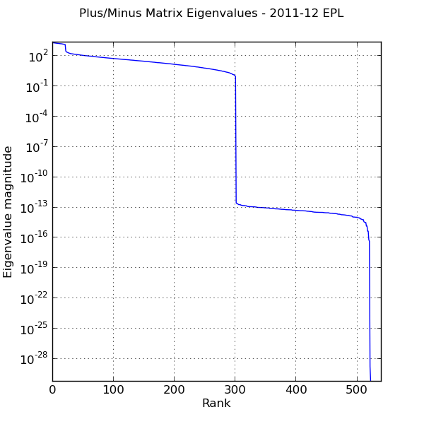
Eigenvalue spectrum of system matrix used in adjusted plus/minus calculation.
At best, half of the eigenvalues in the original system matrix are zero or very very close to it. Little wonder that the resulting parameters are so unstable.
Ridge regression
I said before that ridge regression seeks to balance noise suppression and loss of information in the estimate. I trained the adjusted plus/minus model for various values of \(\lambda\) and selected the one that minimized the RMSE of the test data set. Below is the plot:
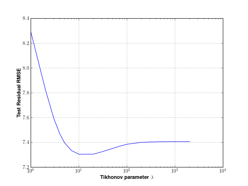
Root-mean-square error of APM test dataset as function of Tikhonov parameter \(\lambda\).
On the basis of this result, I selected \(\lambda^* = 10\).
Here are the top twenty players (2011-12 Premier League) in terms of APM using the optimal ridge regression settings:
| Player | APM / 90 |
| Jonny Evans | 1.069 |
| Leon Best | 0.807 |
| Tom Cleverley | 0.768 |
| James Perch | 0.719 |
| Michael Williamson | 0.687 |
| Mikel Arteta | 0.568 |
| Thomas Vermaelen | 0.539 |
| Edin Džeko | 0.519 |
| Gary Gardner | 0.492 |
| Lucas Leiva | 0.491 |
| Alexandre Song | 0.477 |
| Ashley Young | 0.465 |
| Aleksandar Kolarov | 0.454 |
| Chris Smalling | 0.443 |
| Danny Murphy | 0.443 |
| Emmanuel Adebayor | 0.431 |
| David Vaughan | 0.430 |
| Ryan Giggs | 0.422 |
| Gaël Clichy | 0.421 |
| James Milner | 0.405 |
And the bottom twenty players:
| Player | APM / 90 |
| Joe Allen | -0.458 |
| Bradley Orr | -0.472 |
| Johan Djourou | -0.478 |
| Pablo Zabaleta | -0.490 |
| Sammy Ameobi | -0.490 |
| Francis Coquelin | -0.491 |
| Hugo Rodallega | -0.513 |
| David Jones | -0.522 |
| Chris Martin | -0.532 |
| Stephen Kelly | -0.546 |
| Adam Johnson | -0.550 |
| Nigel de Jong | -0.571 |
| Jay Spearing | -0.576 |
| Hatem Ben Arfa | -0.582 |
| Sebastián Coates | -0.590 |
| Michael Kightly | -0.590 |
| Henri Lansbury | -0.593 |
| Andrew Johnson | -0.605 |
| Anderson | -0.912 |
| Rio Ferdinand | -1.032 |
There are a few caveats with these figures. First, I did not remove players who played less than a certain threshold of minutes. (Any threshold is going to be arbitrary and I couldn’t settle on a number. I’m open to ideas.) Second, there is no standard error, and that is an artifact of the ridge regression method. The biasing that it introduces makes it difficult to calculate a standard error. Perhaps bootstrapping could aid in developing error estimates.
In contrast to the original system matrix, the eigenvalue spectrum of the regularized matrix (figure below) is better behaved. The Tikhonov parameter raises the floor of the spectrum and thus makes all of the eigenvalues nonzero and positive.
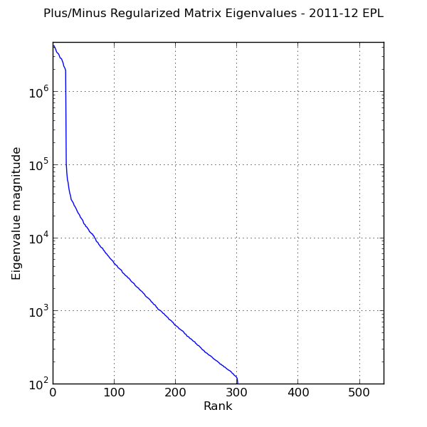
Eigenvalue spectrum of regularized system matrix used in adjusted plus/minus calculation. \(\lambda = 10\).
Is Adjusted Plus/Minus Useless?
So I’ve written about why adjusted plus/minus is challenging to implement and solve. But do the results really matter?
I think the value of adjusted plus/minus in sports like basketball and ice hockey is that there are a lot of segments in both matches, so there are more opportunities to identify those players who have significant impact on the score through their presence. Therefore the top players for that metric are those who everyone would expect — LeBron James, Dwight Howard, Sidney Crosby, Pavel Datsyuk, and so on. Even so, models in either sport can explain 0.1-15% of the variance in the output data.
In football, there is an average of five or six segments in a match, so there are much fewer opportunities to identify big impact players. The out-of-sample prediction for the soccer adjusted plus/minus had a \(R^2 = 0.03\), which meant that 3% of the variance in the goal difference data can be explained by the model. That’s not good and it makes me very skeptical that adjusted plus/minus could be a suitable predictor. However, the figure is in line with similar models in other sports. One remedy is to collect match data from the previous two or three seasons. Another is to employ a cutoff for players with small amount of minutes played, but researchers such as Wayne Winston have shown that those minor players have significant impacts on the plus/minus coefficients of major players. Standard error has to be calculated in order to determine whether the values mean anything. Statistical bootstrapping could have a role to play here.
Adjusted plus/minus in football could become a valuable metric over time, but it will require a lot of care in its formulation, implementation, and interpretation.
